This page is out of date

You've reached a page on the Ren'Py wiki. Due to massive spam, the wiki hasn't been updated in over 5 years, and much of the information here is very out of date. We've kept it because some of it is of historic interest, but all the information relevant to modern versions of Ren'Py has been moved elsewhere.

Some places to look are:

• The Ren'Py Home Page
• Download the Latest Version
• Ren'Py Documentation
• Quickstart Tutorial
• Ren'Py Cookbook

Please do not create new links to this page.

---

Additional basic move profiles

Ren'Py comes with a few basic pre-defined move profiles. The “move” family (“move”, “moveinright”, “moveoutbottom”, etc.) is a simple linear interpolation between the start and end points. The “ease” family (“ease”, “easeinright”, “easeoutbottom”, etc.) uses a cosine curve to create a smooth acceleration/deceleration. The graph below shows what these profiles look like.

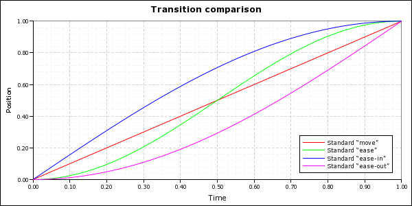
Here are a few additional basic movement profiles that you can use to add some variation to your game.

How to use these functions

The most straightforward way to use these functions is to use them as the time_warp parameter in a call to Move.

init:
  python hide:
    def bop_time_warp(x):
      return -23.0 * x**5 + 57.5 * x**4 - 55 * x**3 + 25 * x**2 - 3.5 * x

start:
  # Move the ball from the left side of the screen to the right with a “bop” profile
  show ball at Move((0.25, 0.5), (0.75, 0,5), 1.0, time_warp=bop_time_warp, xanchor="center", yanchor="center")

You can also use to create a whole new family of transitions using these profiles.

init:
  python hide:
    def quad_time_warp(x):
      return -2.0 * x**3 + 3.0 * x**2
    
    def quad_in_time_warp(x):
      return 1.0 - (1.0 - x)**2
    
    def quad_out_time_warp(x):
      return x**2
    
    define.move_transitions("quad", 1.0, quad_time_warp, quad_in_time_warp, quad_out_time_warp)

start:
  show eileen happy with quadinleft

Quadratic motion

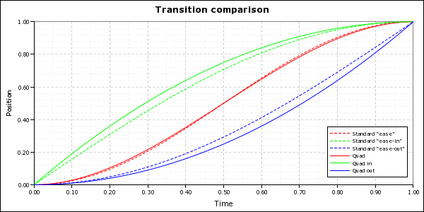
Quadratic motion serves pretty much the same purpose as the standard, cosine-based “ease” motions, but they’re a little more efficient. They’re also a better model for natural accelerations and decelerations, because most natural accelerations (and decelerations) are pretty well modelled as constant acceleration motion, which is quadratic. You can see from the picture that they’re also a little “gentler” - with a less aggressive acceleration/deceleration profile (except the double-ended version, which is a best fit polynomial to a quadratic acceleration followed by deceleration). It may look a bit more organic than the built-in “ease” motion.

def quad_time_warp(x):
  return -2.0 * x**3 + 3.0 * x**2

def quad_in_time_warp(x):
  return 1.0 - (1.0 - x)**2

def quad_out_time_warp(x):
  return x**2

Exponential decay

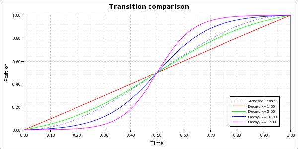
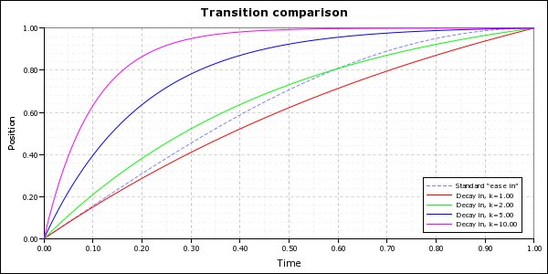
Besides quadratic (constant acceleration) motion, the other most common (non-oscillatory) motion you see naturally is exponentially decaying motion. This is the kind of motion you see when something is being slowed down by friction. They’re much less efficient than the quadratic or standard ease functions, but they also allow you much more control because you can adjust the decay constant k. Larger k values mean the decay is faster (which means a more aggressive acceleration/deceleration profile).

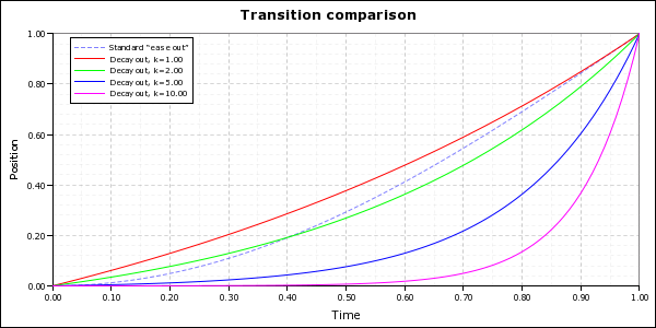
import math

def decay_time_warp_real(x, k):
  return (1.0 / (1.0 + math.exp(-k * (x - 0.5))) - 1.0 / (1.0 + math.exp(k / 2.0))) /
         (1.0 / (1.0 + math.exp(-k / 2.0)) - 1.0 / (1.0 + math.exp(k / 2.0)))

def decay_in_time_warp_real(x, k):
  return (math.exp(1.0) - math.exp(1.0 - k * x)) / (math.exp(1.0) - math.exp(1.0 - k))

def decay_out_time_warp_real(x, k):
  return (math.exp(k * x) - 1.0) / (math.exp(k) - 1.0)

decay_time_warp = renpy.curry(decay_time_warp_real)
decay_in_time_warp = renpy.curry(decay_in_time_warp_real)
decay_out_time_warp = renpy.curry(decay_out_time_warp_real)

Handling the extra parameter

Because of the extra k parameter, you have to use these functions a little differently:

show ball at Move((0.25, 0.5), (0.75, 0,5), 1.0, time_warp=decay_time_warp(k=10.0), xanchor="center", yanchor="center")

# Or...

$ define.move_transitions("decay10", 1.0, decay_time_warp(k=10.0), decay_in_time_warp(k=10.0), decay_out_time_warp(k=10.0))
show eileen happy with decay10inleft

Optimizing

Now, if you pick a k-value and like it, it’s kind of a waste to do all of these calculations every time. You can simplify the equations like this:

import math

def decay_fixed_time_warp(x):
  return AAA / (1.0 + math.exp(-k * (x - 0.5))) - BBB

def decay_fixed_in_time_warp(x):
  return CCC - DDD * math.exp(1.0 - k * x)

def decay_fixed_out_time_warp_real(x):
  return EEE * math.exp(k * x) - EEE

Where:

• AAA:

• BBB:

• CCC:

• DDD:

• EEE:

And don’t forget to set k!

To automate all of this, check out the handy helper script.

Power functions

If you want more control over the acceleration profile – like if you want a more or less aggressive acceleration profile – and you don’t want to pay the price for decay functions, power functions are a cheap substitute.

Note: i made incoming and outgoing versions, but not double-ended ones, because i don’t know a polynomial sigmoid function off the top of my head. A Taylor series expansion of a sigmoid function would work. i thought about the Taylor series expansion of the Error function, but if anyone knows a Taylor series expansion of the Heaviside (step) function between −½ and ½ – not a Fourier series! – that would be perfect.

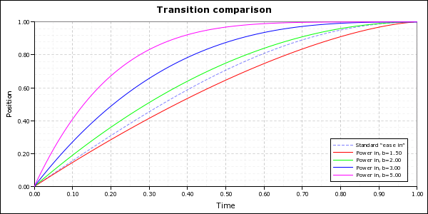
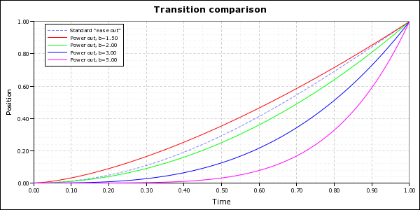
def power_in_time_warp_real(x, b):
  return 1.0 - (1.0 - x)**b

def power_out_time_warp_real(x, b):
  return x**b

power_in_time_warp = renpy.curry(power_in_time_warp_real)
power_out_time_warp = renpy.curry(power_out_time_warp_real)

Tip: If you want a really cheap deceleration profile, a quick and dirty hack is to pass a value greater than zero but less than one to power_out_time_warp. It won’t give you a very pretty profile, but it will give you a very efficient one.

Animation “bop”

This next profile is not so much about modelling reality as it is fun. Next time you watch a kid’s cartoon – Disney stuff is a good example – watch carefully how characters move. If a character is looking down, and then someone calls her, she doesn’t just lift her head. What she does is kind of pull down, then look up. They do this for pretty much every motion they make – they kinda pull back, as if they’re storing up energy to spring, then make the motion. Just watch here, and you’ll see – for example, at about 1:00, Goofy is lying down floating in mid-air, and twice he kinda squeezes in before doing something; at 1:07, it’s a big squeeze, before that is a little one. It’s a silly little thing, but it adds some life to animations.

Each of these “bop” motions overshoots by around 15%. They make your objects either go a bit in the wrong direction before moving in the right direction, or go past where they were supposed to stop then pull back, or both. There are five different profiles. Three match the standard in (“bop in”), out (“bop out”) and normal (“bop move”) motions. And then there are two extra motions that either accelerate at the beginning (“to bop”) or decelerate at the end smoothly (“bop to”). You could use this to, for example, have a character at left move from left to centre to get close to a character at right... they accelerate naturally, but then skid to a stop, realize they’re too close and pull back very quickly.

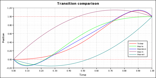
def bop_time_warp(x):
  return -23.0 * x**5 + 57.5 * x**4 - 55 * x**3 + 25 * x**2 - 3.5 * x

def bop_in_time_warp(x):
  return -2.15 * x**2 + 3.15 * x

def bop_out_time_warp(x):
  return 2.15 * x**2 - 1.15 * x

def bop_to_time_warp(x):
  return -5 * x**5 + 5 * x**4 + x**2

def to_bop_time_warp(x):
  return -5 * x**5 + 20 * x**4 - 30 * x**3 + 19 * x**2 - 3 * x

You can use bop_time_warp, bop_in_time_warp and bop_out_time_warp in . bop_to_time_warp and to_bop_time_warp are handy by themselves when you want the motion to start with a bop but end smoothly, or start smoothly but end with a bop.

See also

• Transitions
• Move